Example acoustic features on a logarithmic frequency axis

SHARK audio frontend

Decoupling sample-rate from sequence length

Julian C. Schäfer-Zimmermann

Max Planck Institute of Animal Behavior

Department for the Ecology of Animal Societies

Communication and Collective Movement (CoCoMo) Group

Bioacoustics spans frequency scales

The frequency band of interest changes across taxa—and across questions.

Sample rate f_s 16 kHz

Nyquist limit f_s / 2 8 kHz Ideal upper boundary

Raw mono, 16-bit PCM 115.2 MB/h 1× the data at 16 kHz

Speech: the G.722 passband is below Nyquist.

A speech-processing convention; other speech applications use wider bands.

Preserve the frequencies the question needs.
Higher sample rates increase raw data for every recorded second.

Enable JavaScript to explore the frequency chart.
Fin-whale note: 18–23 Hz; G.722 speech passband: 50 Hz–7 kHz;
great-tit notes: 2.4–5.3 kHz; bat harmonics: 22–105 kHz;
dolphin click plateau: 40–120 kHz; katydid carrier: ≈150 kHz.

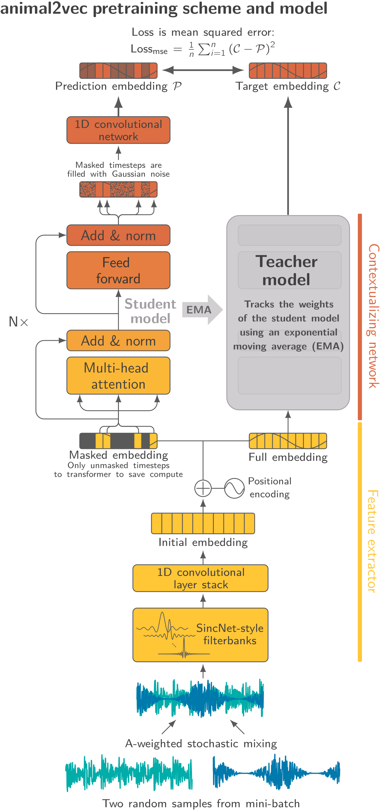
animal2vec

Learning useful representations from large amounts of bioacoustic data.

Raw audio

The recorded waveform

Frontend

Extracts short, local acoustic features

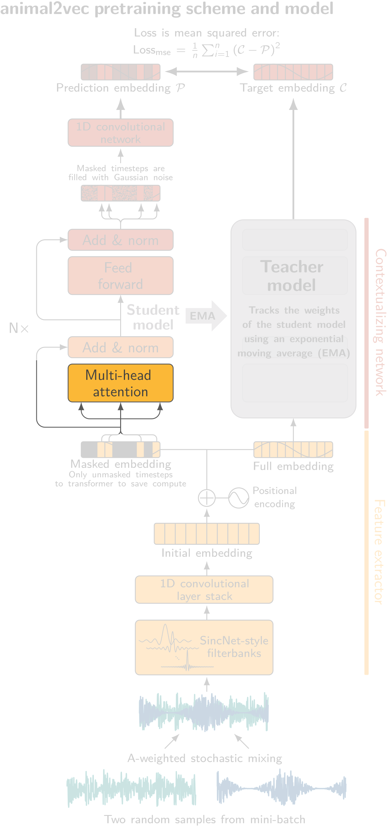
Transformer
Self-attention blocks

Main contextual
feature extraction

Task head

Detects and classifies calls

Pretrain: predict masked representations from the surrounding audio.
Fine-tune: use annotations to learn the task.

The frontend determines how much work
reaches the self-attention blocks.

Schäfer-Zimmermann et al., Methods Ecol. Evol. (2026). doi:10.1111/2041-210x.70218

animal2vec learns acoustic representations before we ask it to solve a labelled task. A learned frontend first extracts local acoustic features. The large Transformer, built around self-attention blocks, is where these local features become contextual representations. This is the computationally demanding stage we want to make more affordable. I am deliberately keeping its internal mechanism for the next slide.

During self-supervised pretraining, a student processes a masked feature sequence and predicts contextual target representations from a teacher that sees the complete sequence. The training target is a learned representation, not the missing raw waveform. Fine-tuning adds the supervised detection/classification objective. The task head shown here is the downstream use, not the full pretraining architecture.

Precision: the frontend also learns features, and Transformer blocks include feed-forward layers as well as attention. “Main contextual feature extraction” is a conceptual description, not a measured fraction of information or parameters.

Source: animal2vec and MeerKAT, final article, §2.2.1 and Figure 3, https://doi.org/10.1111/2041-210x.70218. Frontend details also appear in https://arxiv.org/html/2406.01253v2, §IV.4.

animal2vec

Quadratic Complexity in Attention: $O(N^2)$

Tokens ($N$): 5

Dot products ($N^2$): 25

Sample Rate vs. Sequence Length

Illustration for a frontend with a fixed stride in samples.

Sampling Rate ($f_s$): 12 kHz

Sequence Token Count ($N$): 6

Attention Matrix ($N^2$): 36

Signal $x(t)$

Example

$\text{N} = 3 \cdot 96,000 = 288,000$

Example

$\text{N} = 3 \cdot 4,000 = 12,000$

A reduction of $576$ in attention matrix size

Heterodyning

Some math ... sorry

Heterodyning

Assuming two signals:

\[ S_1(t) = A_1 \cos(\omega_1 t) \]

\[ S_2(t) = A_2 \cos(\omega_2 t) \]

$ S_1(t)$ is the signal we want to downshift

$ S_2(t)$ is the signal we use for downshifting $ S_1(t)$

Heterodyning

Heterodyning is defined as the mathematical product of these two time-domain signals:

\[ S_{\text{out}}(t) = S_1(t) \cdot S_2(t) \]

Substituting the signal functions:

\[ S_{\text{out}}(t) = A_1 A_2 \cos(\omega_1 t) \cos(\omega_2 t) \]

Heterodyning

To resolve the frequency components, apply the trigonometric product-to-sum identity:

\[ \cos(\alpha) \cos(\beta) = \frac{1}{2} \left[ \cos(\alpha - \beta) + \cos(\alpha + \beta) \right] \]

Substituting $\alpha = \omega_1 t$ and $\beta = \omega_2 t$.

Heterodyning

Expanding the terms maps the output into two distinct frequencies:

\[ S_{\text{out}}(t) = \frac{A_1 A_2}{2} \left[ \cos\left( (\omega_1 - \omega_2)t\right) + \cos\left( (\omega_1 + \omega_2)t \right) \right] \]

Heterodyning

The system maps the original frequencies to two new spectral coordinates:

Difference Frequency (Intermediate Frequency / IF): \[ \omega_{\text{IF}} = |\omega_1 - \omega_2| \] Utilized for down-conversion workflows.
Sum Frequency (Up-conversion): \[ \omega_{\text{sum}} = \omega_1 + \omega_2 \] Typically eliminated via lowpass or bandpass filtering.

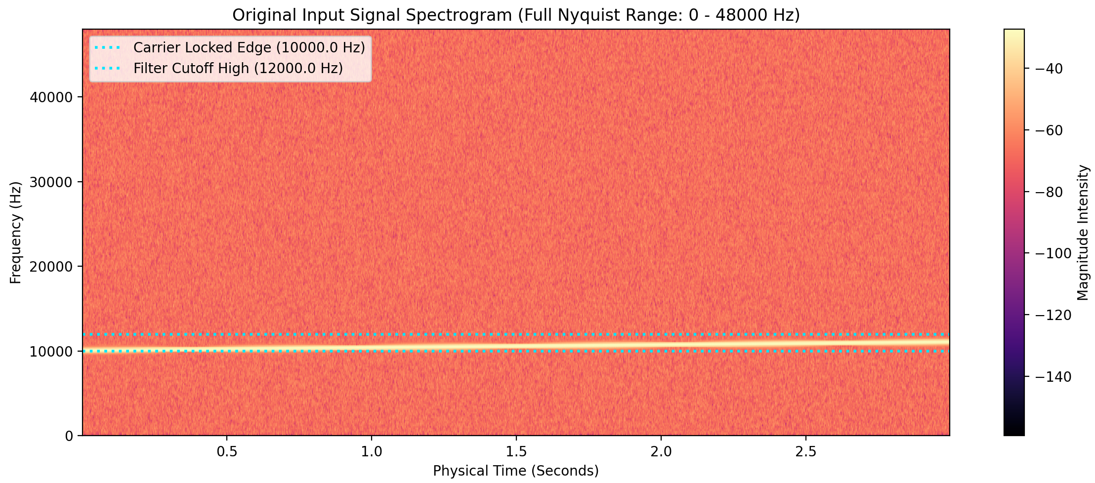
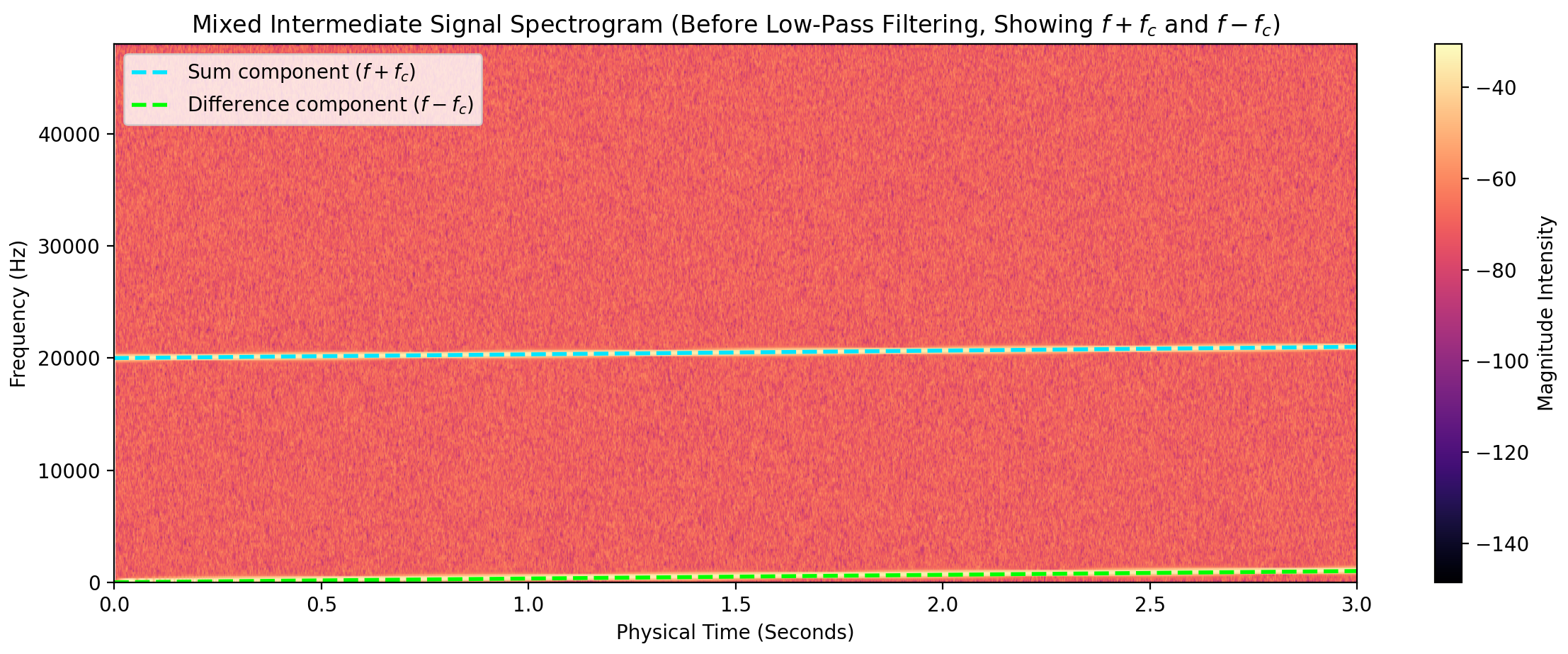
Example

We multiply by a 10 kHz signal to shift the frequency band

Example

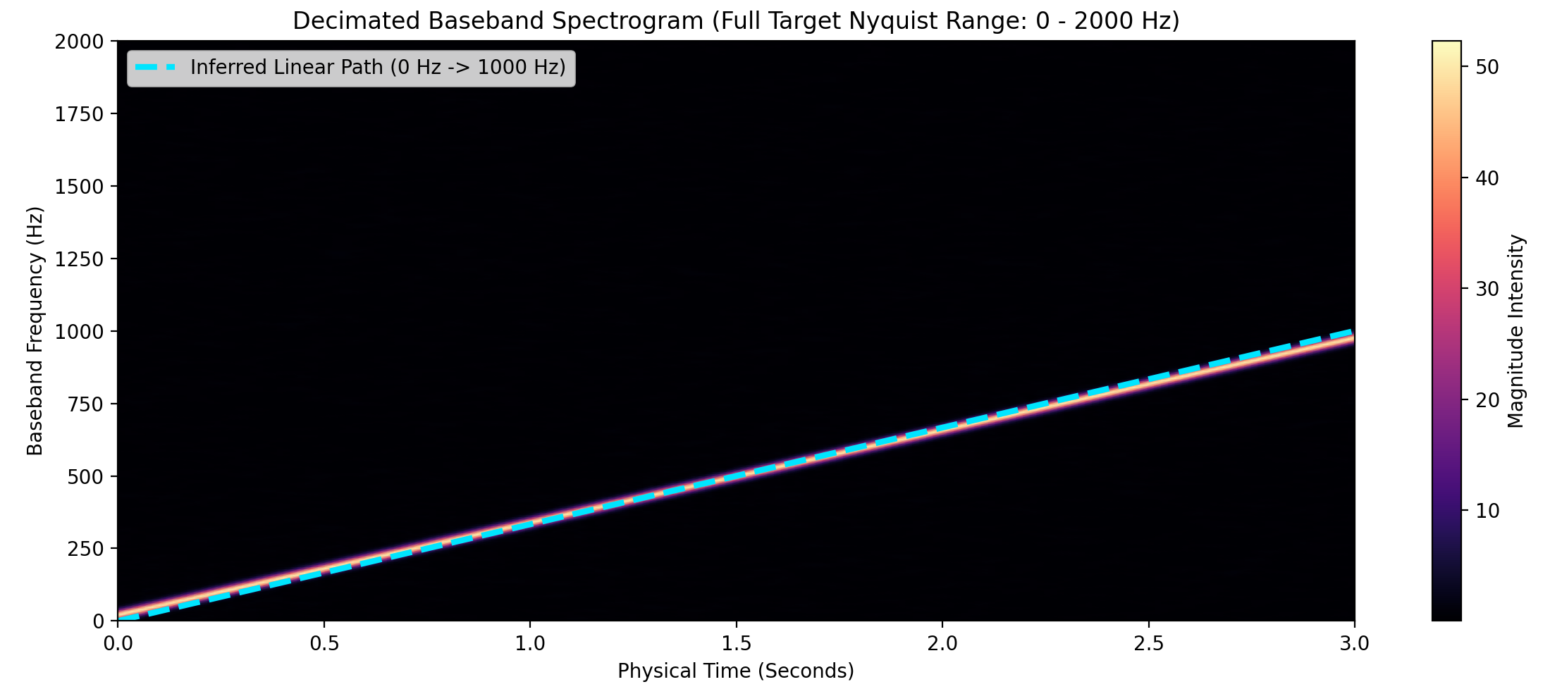
Up- and downshifted components $\Rightarrow$ Low-pass filter, then downsample

Example

Only the low-pass-filtered, downshifted component remains

The SHARK frontend

Turn each frequency band into
a slowly varying amplitude signal.

1Choose bands

Use the same physical frequency map.

2Shift down

Heterodyne each band to baseband.

3Follow amplitude

Filter and extract the band envelope.

4Share a clock

Anti-alias filter, then sample at 250 Hz.

8 kHz input

48 kHz input

192 kHz input

Equal duration, equal time axis. Band counts are schematic. Fixed operations, no learned weights.

Higher input rates add valid frequency bands.
The temporal grid stays fixed.

The heterodyning example showed how one frequency region can be shifted down. SHARK repeats this across a shared bank of bands. After quadrature mixing and low-pass filtering, it extracts an envelope-like energy feature. A second anti-alias filter allows the band signals to be converted to a common rate of 250 samples per second. Their physical band identities are retained as channels.

All recordings use the same band map within a configured model. Bands above a recording's Nyquist limit are masked. The output is a band-by-time representation, followed by log compression and temporal normalization (LogTBN). The diagrams show coverage only; the number of depicted rows is deliberately not proportional to the number of actual bands.

The displayed 250 Hz is the output sampling rate of each band, not the original recording rate. The frontend description on p. 4 also specifies a nominal 250-Hz band bandwidth; these are different quantities. Envelope extraction discards waveform phase and is not lossless reconstruction. Higher input rates still cost more frontend processing and may expose more bands; only the temporal grid is independent of input rate for fixed duration and configuration.

Sources: supplied SHARK draft v0.5, Fig. 1 (p. 4), frontend description (pp. 4–5), Table 5 (p. 12).

Other frontends

PteroSet: three controlled conditions

The same bird recordings and labels, three audio variants.

Shared 48 kHz192 kHz → 48 kHz	Standard performance Can SHARK compete when every recording has the same rate?
Upsampled 48–192 kHz48 kHz → higher stored rates	Redundant sampling Does performance change when we add sample points without adding acoustic information?
Mixed 8–192 kHz192 kHz → varying target rates	Changing rate and bandwidth Can one frontend handle recordings with different available frequency content?

Fixed data variants. Same ~2M-parameter Transformer for every frontend.
Binary vocalization detection in 5-second examples.

Separate redundant sampling from changes in bandwidth.

PteroSet: Ruiz et al. (2026).

PteroSet lets us change the representation of the audio without changing the underlying recording collection or annotations. The first condition is the conventional 48-kHz dataset recommended by its authors. In the second, we first create that same 48-kHz signal, then store it at randomly selected rates from 48 to 192 kHz. This adds sample points but no new recorded information. The third starts from the original 192-kHz recordings and resamples them to rates between 8 and 192 kHz, so available bandwidth also changes.

Variants are prepared and fixed before training. The common Transformer has two layers, 256-dimensional embeddings and four heads, approximately two million parameters. The frontends are SHARK minimal, log-Mel, LEAF and Conv1D. The experiment evaluates binary vocalization presence, not bird-species identity.

Evaluation uses the MAP1 validation split, not a five-fold average or a separately identified held-out test set. Sequence AP uses five non-overlapping windows per 5-second example. A separate frame-level AP interpolates outputs to a common 1-ms grid.

Qualification: these are performance comparisons across separately prepared training conditions, not proof that representations are exactly identical for paired waveforms. The SHARK bank configuration also differs between the shared and mixed conditions. The draft's accuracy sections do not unambiguously specify whether the conventional frontends use fixed sample-domain hops or rate-normalized physical hops, so no conclusion about that specific choice is attached here.

Sources: PteroSet: Ruiz et al., arXiv:2605.20578.

PteroSet: highest AP in all three conditions

Average precision (AP). Higher is better.

Frontend	Shared 48 kHz	Upsampled 48–192 kHz	Mixed 8–192 kHz
1-second prediction windows
SHARK minimal	0.826	0.788	0.795
log-Mel	0.673	0.419	0.537
LEAF	0.624	0.646	0.630
Conv1D	0.619	0.587	0.595
Frame predictions on a shared 1-ms evaluation grid
SHARK minimal	0.585	0.525	0.561
log-Mel	0.377	0.175	0.295
LEAF	0.429	0.412	0.265
Conv1D	0.381	0.319	0.295

MAP1 validation. Shared ~2M backbone. The 1-ms grid interpolates predictions.

SHARK minimal leads on both readouts.

The main result is consistent across both readouts: SHARK minimal has the highest AP in each condition. For one-second windows, its AP is 0.826, 0.788 and 0.795. The advantage over the best conventional baseline in each column is 15.3, 14.2 and 16.5 AP points.

Frame AP gives the same ranking at the top. The corresponding advantages over the best baseline are 15.6, 11.3 and 26.6 points. An AP point here means 0.01 absolute AP, not a relative percent change.

These results support strong performance across the three prepared conditions, not exact empirical invariance. Within SHARK, upsampling changes sequence AP by -0.038 and frame AP by -0.060. Other frontends can show smaller changes in some comparisons, so do not claim that SHARK has the smallest degradation in every case. No uncertainty intervals or repeated-run variability are reported for these accuracy values.

AP summarizes the precision–recall tradeoff across thresholds. It is not the percentage of correctly classified examples. The source calls the upper readout sequence predictions: five non-overlapping windows per 5-second example, i.e. one-second windows.

Source: supplied SHARK draft v0.5, Table 1 and evaluation description (p. 8). Numeric AP values are reproduced without the draft's erroneous relative-percentage annotations.

Mixed rates across animal datasets

Can one model learn from recordings spanning
8–250 kHz and very different acoustic environments?

MeerKAT8 kHzMeerkats

HyenaSET24 kHzHyenas

PteroSet48 kHzBirds

Neotropical
katydids96 kHzInsects

Egyptian
fruit bats250 kHzBats

One task: detect animal vocalizations over time.

45.3 hours in total. Corpus-specific input rates. Shared ~125M Transformer.
Compare all frontends, including SHARK minimal and enhanced.

A test of joint learning across heterogeneous recordings.
Rate, taxon and recording conditions vary together.

PteroSet uses its prepared 48-kHz variant.

The PteroSet comparison changes sample rate within one recording domain. This next benchmark asks whether a single shared frontend and Transformer can learn from recordings whose sample rate, species, sensor and environment all differ. We combine about ten hours from each of five corpora, except the katydids, where about four and a half hours of labelled audio are available.

The common task is deliberately simple: animal-vocalization presence versus background at each time point. It is not five-class taxon recognition or a common call-type taxonomy. Original onset and offset times are retained. Uncertain annotation regions are excluded from the loss.

The five rates are 8, 24, 48, 96 and 250 kHz, a 31.25-fold range. PteroSet uses the previously downsampled 48-kHz variant, so “all original native recording rates” would be an overstatement. Input examples are 5 seconds. The common backbone has 12 layers, 768-dimensional embeddings and 12 heads, approximately 125 million parameters. Enhanced adds extra stem modules, so common backbone does not imply identical total parameter counts.

Interpretation: sample rate is confounded with taxon and recording domain. This is a realistic joint-learning stress test, not an isolated causal test of sampling-rate invariance. The controlled PteroSet comparisons address the latter more directly.

Mixed rates: enhanced SHARK leads overall

Frame-level average precision (AP). Higher is better.

Dataset	SHARK minimal	SHARK enhanced	log-Mel	LEAF	Conv1D
Micro AP	0.404	0.779	0.564	0.253	0.199
Macro AP	0.274	0.629	0.435	0.256	0.318
MeerKAT	0.553	0.846	0.310	0.166	0.240
HyenaSET	0.483	0.859	0.639	0.345	0.603
PteroSet	0.108	0.423	0.259	0.111	0.074
Katydids	0.066	0.118	0.052	0.058	0.040
Fruit bats	0.161	0.900	0.914	0.601	0.635

Micro: all frames pooled. Macro: mean AP across the five corpora.

+21.5 AP points micro; +19.4 macro over log-Mel.
Enhanced leads on four corpora. Log-Mel leads on fruit bats.

Shared 1-ms evaluation grid. Highlight: highest AP in each row. Absolute AP differences.

Enhanced SHARK gives the strongest aggregate result. Micro AP is 0.779 compared with 0.564 for log-Mel, an absolute gain of 21.5 AP points. Macro AP is 0.629 versus 0.435, a gain of 19.4 points. Macro gives equal weight to each corpus; micro computes AP after pooling the evaluated frame predictions and labels.

The per-corpus results matter. Enhanced leads on four of the five corpora, but log-Mel remains slightly ahead for fruit bats: 0.914 versus 0.900. Katydid AP remains low for every method. SHARK minimal is much weaker overall, so the mixed-rate result should be attributed specifically to the enhanced configuration.

The enhanced configuration changes both cross-band attention and frequency pooling. This comparison does not separately identify the contribution of either component. The common backbone is approximately 125 million parameters, whereas the PteroSet experiments used a roughly 2-million-parameter backbone; values should not be compared across those experiments as if all else were equal.

No confidence intervals or accuracy-run variability appear in the draft. These are numerical comparisons, not a claim of statistical significance. Source: supplied SHARK draft v0.5, Table 3 (p. 10), evaluation description (p. 9).

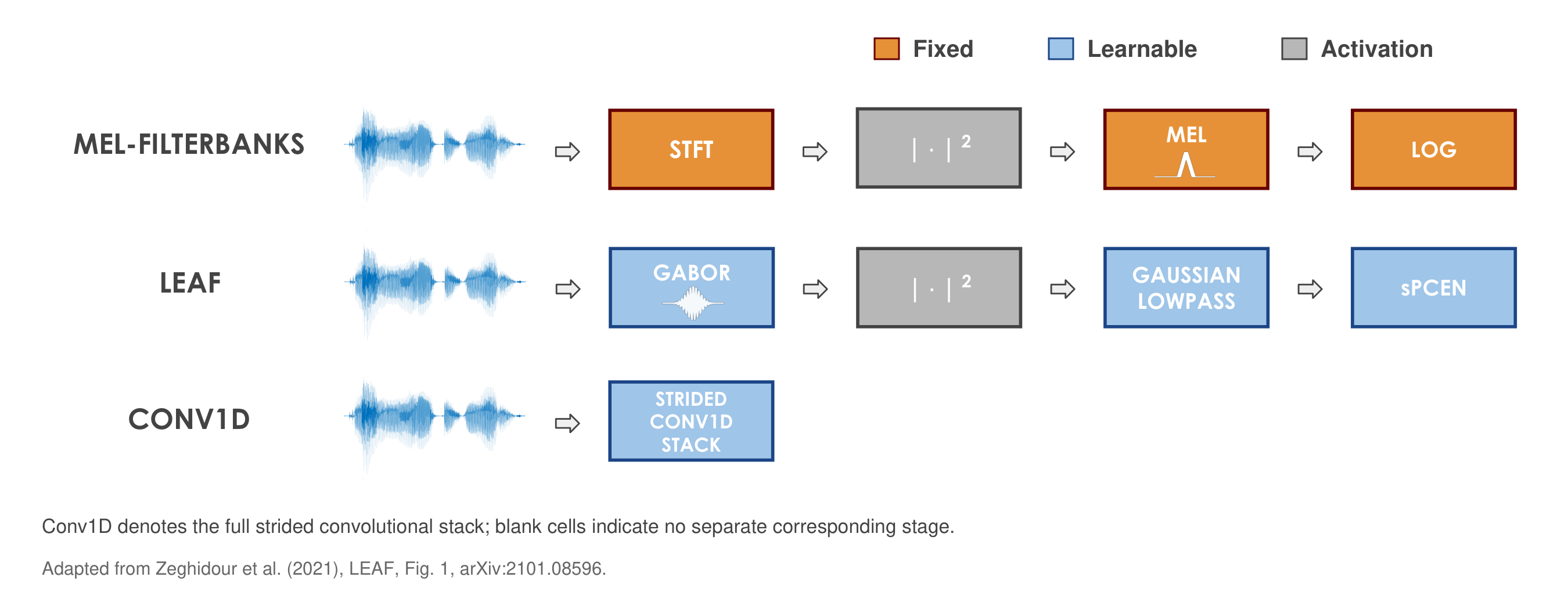
Other frontends

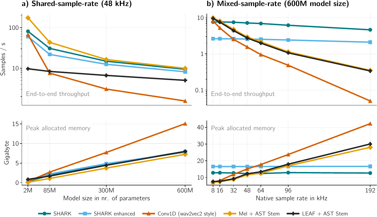
Outlook

Foundation-scale animal2vec

Pretrain on larger collections of animal audio at different sampling rates.

Use a shorter, shared time grid to make larger models and longer context more practical.

Next test: representations that transfer across taxa, environments and tasks.

An electronic frontend

The fixed signal-processing stages could run in dedicated circuitry on the sensor.

Mixing + filtering + envelopes
↓
Low-rate digitization
↓
Digital stem and model

Next: validate feature quality and measure whole-device energy use.

Make large-scale learning more practical,
and bring efficient preprocessing closer to the recording.

The immediate direction is foundation-scale animal2vec training. SHARK removes one computational obstacle: recordings with higher stored rates no longer force a longer temporal sequence into the Transformer. This should make it more practical to combine diverse datasets, use larger backbones and investigate longer behavioural context. Broad transfer from that pretraining remains a next experiment, rather than a result already demonstrated here.

The second direction comes from the fact that the frontend uses fixed signal-processing operations. Quadrature mixers, low-pass filters and envelope extraction could be implemented in analog or mixed-signal circuitry, followed by low-rate digitization. The learned stem and model would remain digital. This could move expensive high-rate preprocessing into dedicated hardware on autonomous recorders or animal-borne sensors.

The draft cites related analog filterbanks as proof of principle, not a completed SHARK circuit. Their band counts and frequency coverage do not establish SHARK-scale ultrasonic feasibility. Next steps include filter response, noise, leakage, temporal alignment, downstream performance and end-to-end power measurements. No device-level energy saving is claimed here.

Compute qualification: the efficiency figure uses minimal SHARK. Fixed temporal sequence length does not remove all frontend costs or the enhanced variant's cross-band attention cost. The current paper's reported evaluations are supervised benchmarks; this outlook proposes the next self-supervised training stage.

Acknowledgments

SHARK is a collaborative project.

Portrait of Marie A. Roch — **Marie A. Roch** San Diego State University

Portrait of Ariana Strandburg-Peshkin — **Ariana Strandburg-Peshkin** Max Planck Institute of Animal Behavior

SHARK audio frontend

Decoupling sample-rate from sequence length

Julian C. Schäfer-Zimmermann

Max Planck Institute of Animal Behavior

Department for the Ecology of Animal Societies

Communication and Collective Movement (CoCoMo) Group