Heterodyning Audiofrontend
Learning to look for the right frequencies
Julian C. Schäfer-Zimmermann
Max Planck Institute of Animal Behavior
Department for the Ecology of Animal Societies
Communication and Collective Movement (CoCoMo) Group

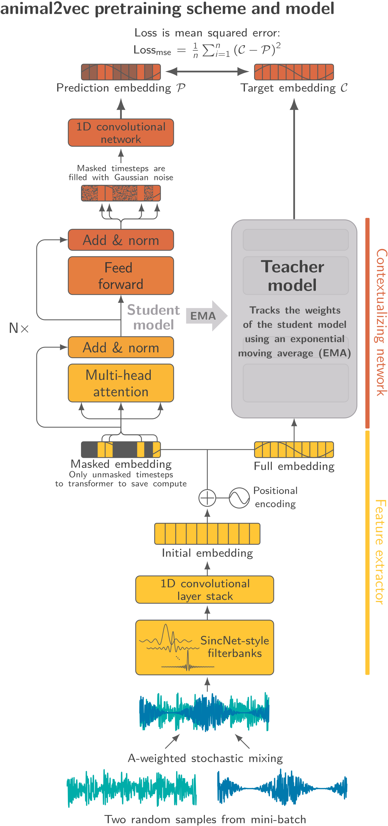
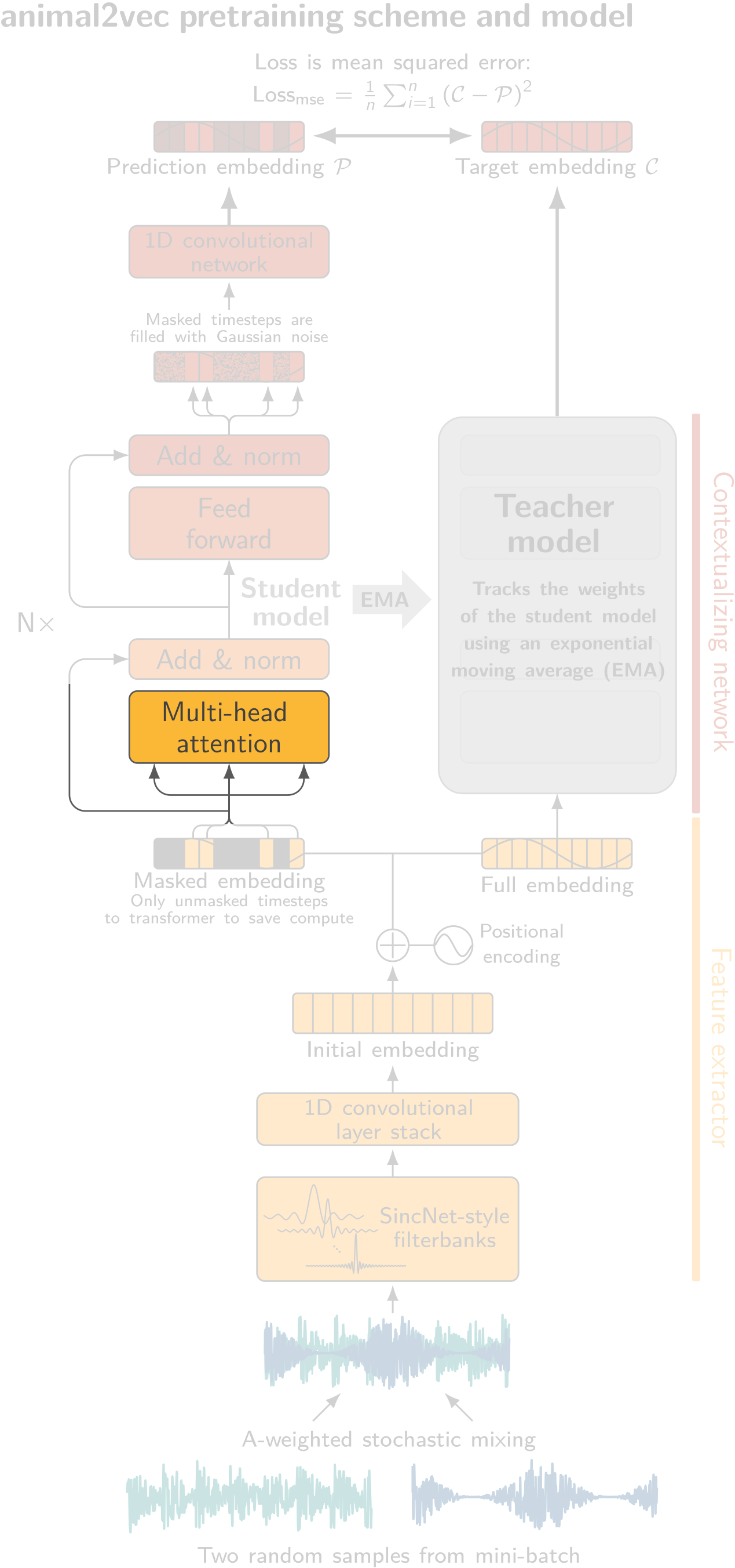
animal2vec
Quadratic Complexity in Attention: $O(N^2)$
Sample Rate vs. Sequence Length
Example
$\text{N} = 3 \cdot 96,000 = 288,000$
Example
$\text{N} = 3 \cdot 4,000 = 12,000$
A reduction of $576$ in attention matrix size
Heterodyning
Some math ... sorry
Heterodyning
Assuming two signals:
\( S_1(t)\) is the signal we want to downshift
\( S_2(t)\) is the signal we use for downshifting \( S_1(t)\)
Heterodyning
Heterodyning is defined as the mathematical product of these two time-domain signals:
Substituting the signal functions:
Heterodyning
To resolve the frequency components, apply the trigonometric product-to-sum identity:
Substituting $\alpha = \omega_1 t$ and $\beta = \omega_2 t$.
Heterodyning
Expanding the terms maps the output into two distinct frequencies:
Heterodyning
The system maps the original frequencies to two new spectral coordinates:
- Difference Frequency (Intermediate Frequency / IF): \[ \omega_{\text{IF}} = |\omega_1 - \omega_2| \] Utilized for down-conversion workflows.
- Sum Frequency (Up-conversion): \[ \omega_{\text{sum}} = \omega_1 + \omega_2 \] Typically eliminated via lowpass or bandpass filtering.
Example
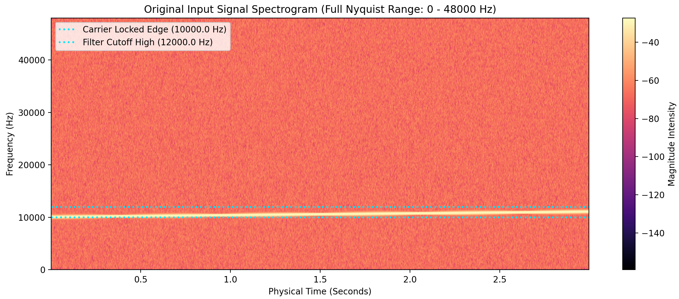
We multiple with a 10 kHz signal for downshifting
Example
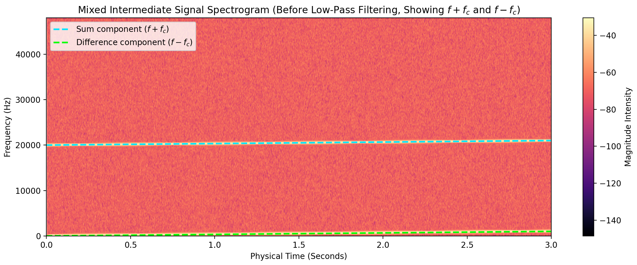
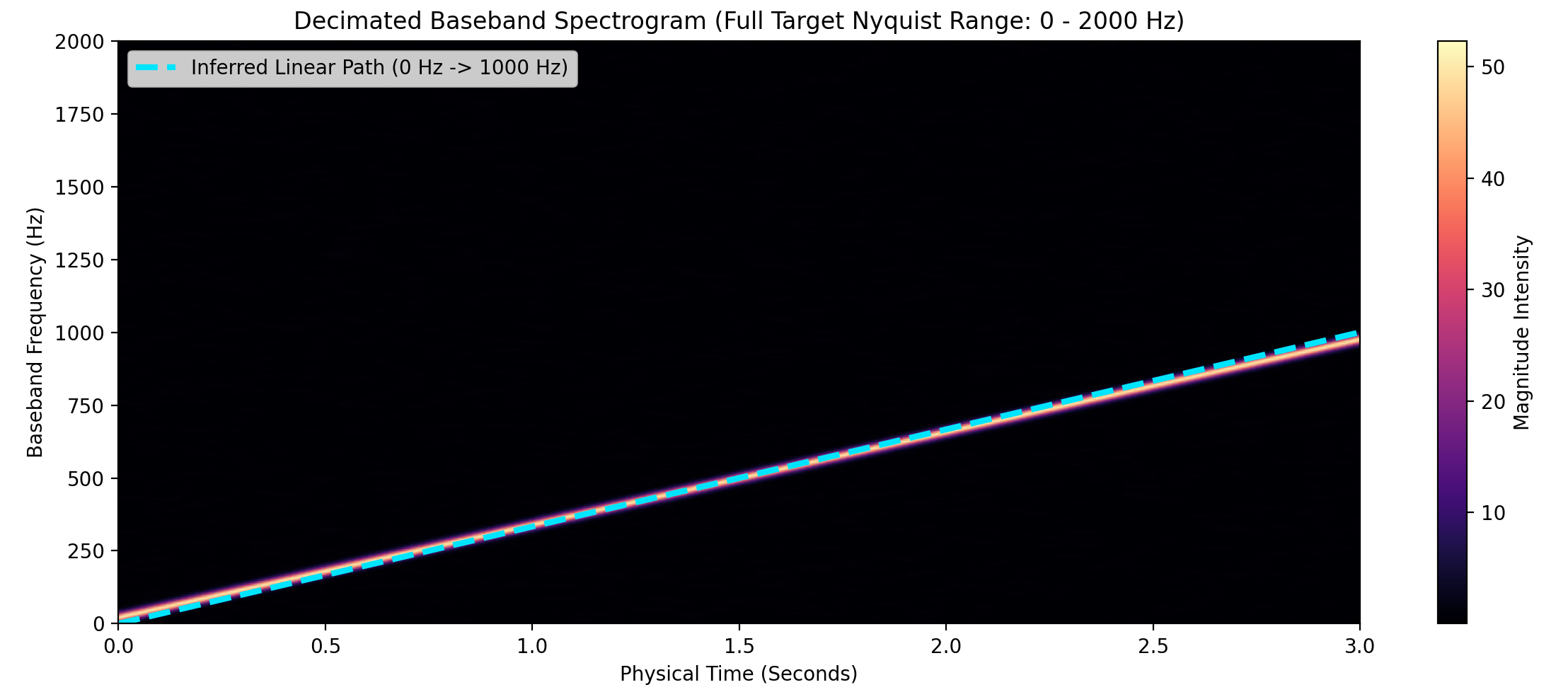
Up- and Downshifted signals are visible $\Rightarrow$ Downsample
Example
Only the downshifted mixture remains
Architecture and test scenario
Look at changes not absolutes
Mathematical Formulation
Power spectrogram from complex STFT $X(f, t)$:
$$P(f, t) = |X(f, t)|^2$$Temporal variance per frequency bin $f$:
$$\sigma_P^2(f) = \text{Var}_t(P(f, t))$$Combined soft Cauchy bandpass mask (soft-OR):
$$M(f) = 1 - \prod_{k=1}^K (1 - M_k(f))$$Transient Energy Coverage Loss
Objective Function
Log-ratio of total variance to captured variance:
$$\mathcal{L}_{\text{energy}_{\text{var}}} = \log\left(\sum_f \sigma_P^2(f)\right) - \log\left(\sum_f M(f) \cdot \sigma_P^2(f) + \epsilon\right)$$Physical Interpretation
- Bypasses static energy (e.g., constant background hums like wind or water).
- Measures energy changes over time ($\sigma_P^2$).
- Forces bandpass filters to target frequency bins containing high-magnitude transient bursts.
Surprise Coverage Loss
Mathematical Formulation
Probability distribution $p(f)$ of temporal variance across the spectrum:
$$p(f) = \frac{\sigma_P^2(f)}{\sum_{f'} \sigma_P^2(f')}$$Information surprise (Shannon entropy component) per bin $f$:
$$S(f) = -p(f) \log(p(f) + \epsilon)$$Total vs. captured spectral entropy:
$$S_{\text{total}} = \sum_f S(f) \quad \text{and} \quad S_{\text{captured}} = \sum_f M(f) \cdot S(f)$$Surprise Coverage Loss
Objective Function
$$\mathcal{L}_{\text{surprise}} = \log(S_{\text{total}}) - \log(S_{\text{captured}} + \epsilon)$$Physical Interpretation
- Maximizes the proportion of spectral entropy captured by the filters.
- If the entire spectrum has a uniform, low-level fluctuation (like wind blowing leaves or moving water), the entropy of that variance is very flat.
- Forces bands to snap onto highly localized, narrow-band peaks (e.g., clean animal calls).
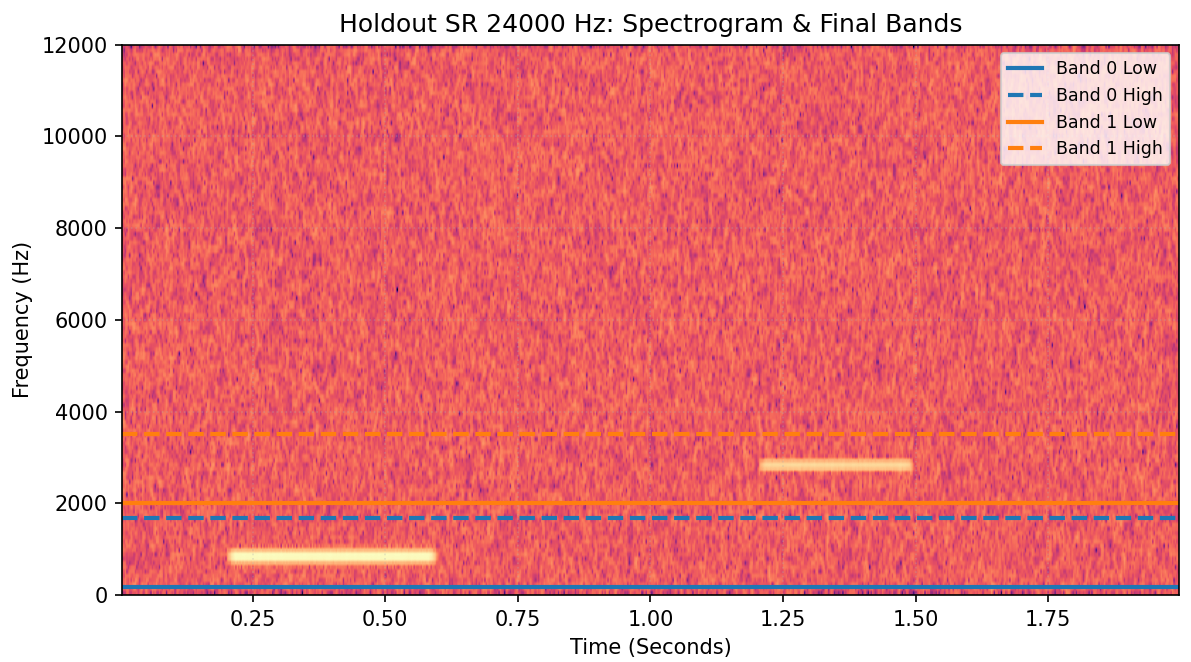
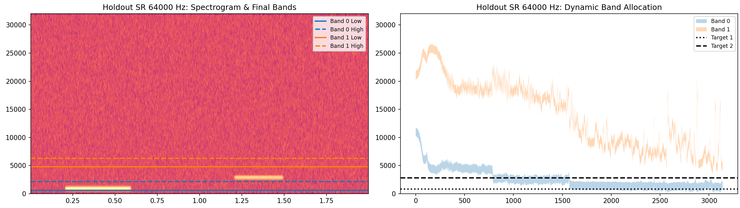
Synthetic dataset
Idealized synthetic bioacoustic dataset:
- Short bursts at various frequencies with varying lengths
- Each input sample has a different sampling rate, but constant length
- Out of: 8000, 16000, 22050, 32000, 44100, 48000 Hz
Eval metrics by sampling rate

Eval metrics by sampling rate
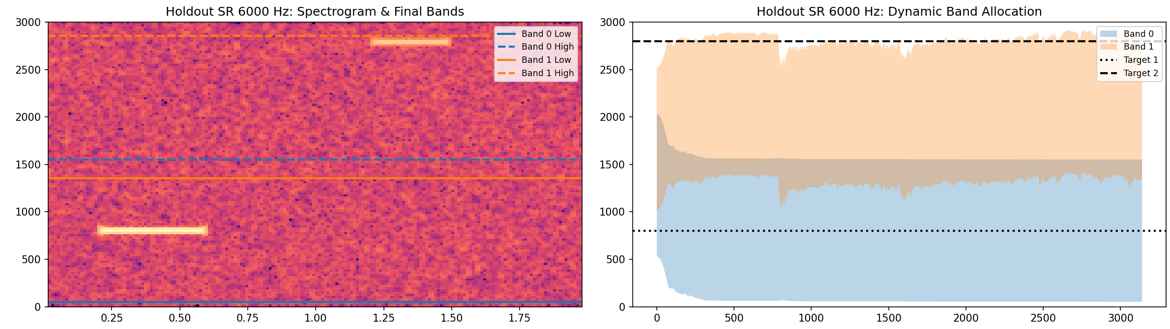
Eval metrics by sampling rate
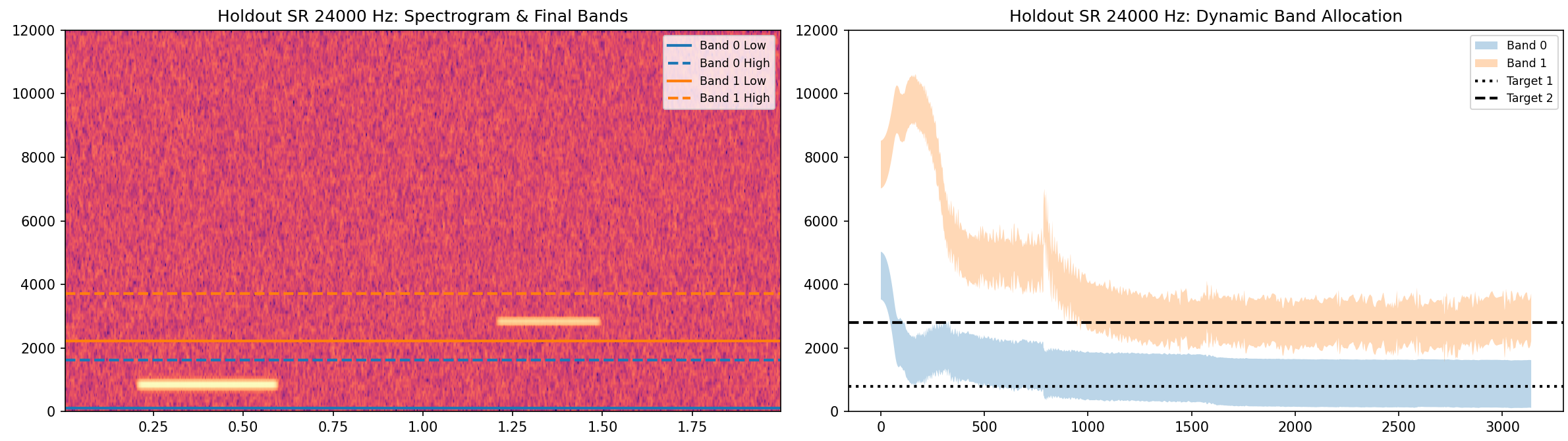
Eval metrics by sampling rate
Summary
- We have an audio frontend that:
- Always outputs a fixed sequence length regardless of the input sample rate
- Is able to find the adequate frequencies on its own in a synthetic benchmark, regardless of the input sample rate
- Is lightweight and faster than other frontends
- What we still have to find out:
- Is it working in a real-life scenario (complex vocalizations with pitch, structure, and harmonics surrounded by a lot of noise)?
- Will it work in a larger pipeline solving complex tasks (e.g., self-supervised self-distillation, as in a2v)?
Heterodyning Audiofrontend
Learning to look for the right frequencies
Julian C. Schäfer-Zimmermann
Max Planck Institute of Animal Behavior
Department for the Ecology of Animal Societies
Communication and Collective Movement (CoCoMo) Group