without math
Department for the Ecology of Animal Societies
Communication and Collective Movement (CoCoMo) Group
Start with the output you need
Where did a call occur?
A start time, an end time, and a label.
What sounds are present?
One or more labels for a recording.
Which examples are similar?
Neighbours in a learned representation.
What should I annotate next?
Candidates for human review.
Choose one of these questions for your own recordings.
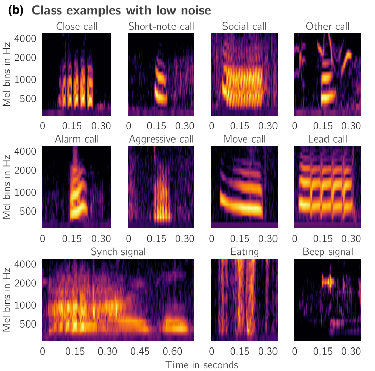
The difficult part is not an isolated clean call
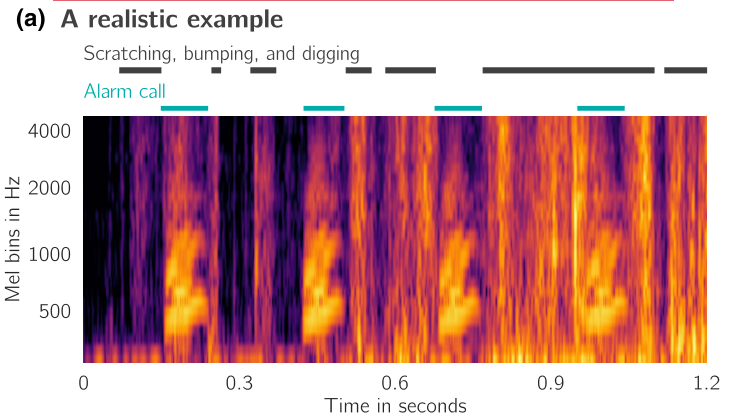
Find the vocalization.
Ignore the recorder.
Keep the timing.
Which strong acoustic events in this figure are not the target vocalizations?
Rare can mean few events—or little time
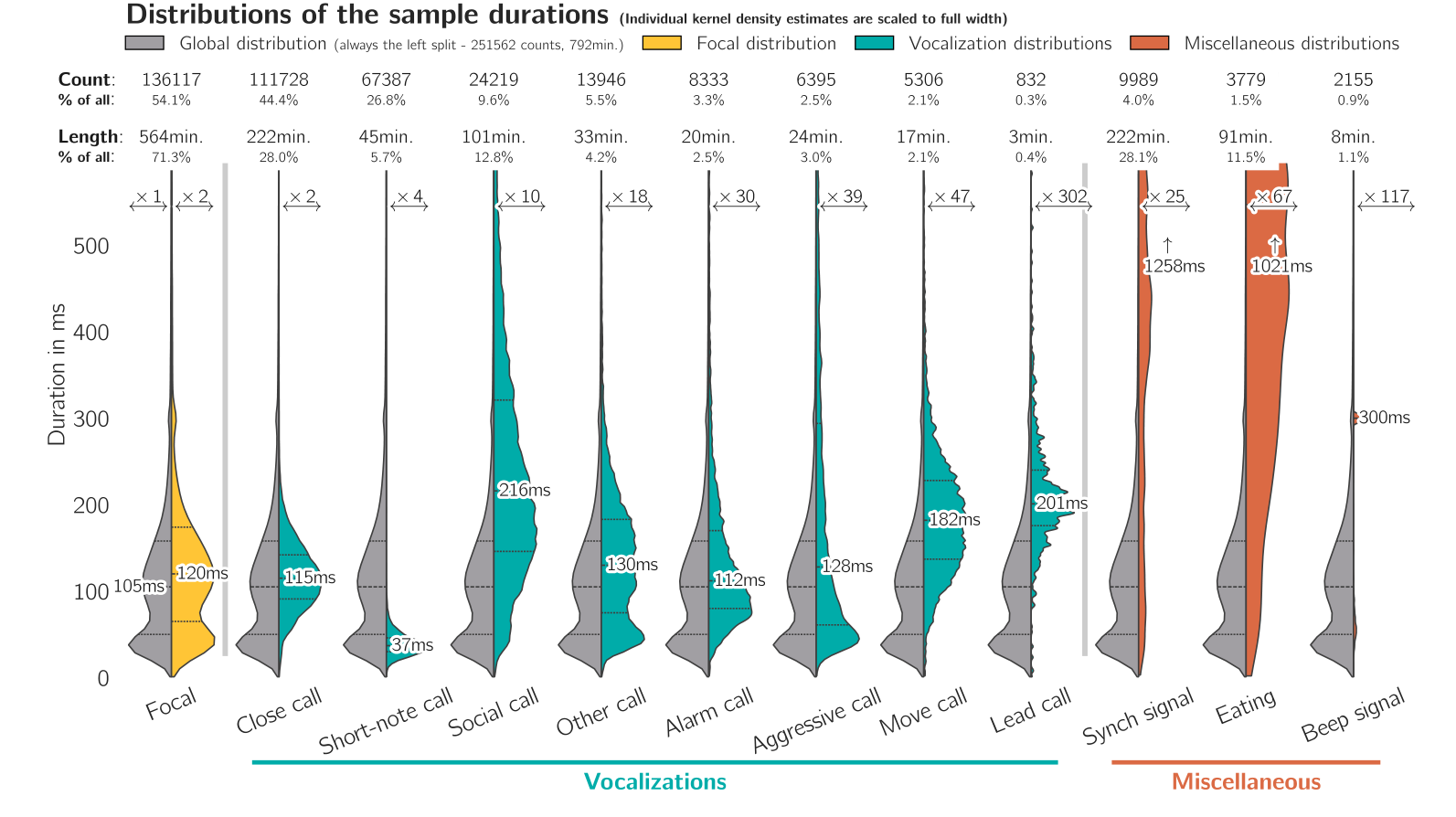
184 h with complete event labels
A short-note call has a median duration of 37 ms.
Learn, specialize, apply
Learn useful representations
Learn the target labels
Apply fixed weights
A neural network is a chain of learned transformations
Before training
The adjustable values do not yet solve the task.
After training
The values have been changed using a training objective.
Training adjusts the model; inference does not
When you run the same checkpoint on a new WAV file, which box is absent?
The input is a waveform—not a picture
amplitude samples per second
10 seconds → 80,000 samples
A spectrogram is a view of the audio
Useful for us to inspect frequencies and timing. It is not the input image expected by this model.
Learned filters turn samples into local features
Look locally first.
A SincNet-style filterbank learns frequency bands. Convolutions turn nearby samples into a shorter sequence of feature vectors.
A feature vector is a list of numbers describing a local part of the signal.
A model frame is not a waveform sample
Local evidence becomes contextual evidence
Local question
What pattern is present around this position?
Contextual question
How does that pattern relate to the rest of this segment?
Attention: which other positions matter here?
Interactive example requires JavaScript.
Move the selected frame. Which parts of the segment could change its interpretation?
An embedding exists before the label decision
Illustration: rows are time positions; columns are learned dimensions.
A description in numbers.
The classification head reads this description and produces scores for the trained labels.
Embedding ≠ call label.
Several labels may be true at the same time
| Output label | Illustrative score | Interpretation |
|---|---|---|
| Close call | 0.82 | Evidence for this call type |
| Alarm call | 0.07 | Little evidence for this label |
| Focal | 0.76 | The caller may be the focal animal |
Illustrative numbers, not measured checkpoint outputs.
Four related outputs, four different questions
| Representation / output | One row or answer per… | What it supports |
|---|---|---|
| Frame scores | Model position × label | When is label evidence high? |
| Fused events | Contiguous active interval | Where does a predicted event start/end? |
| Recording-level labels | Recording × label | Which labels occur somewhere? |
| Embeddings | Model position × feature | How can sounds be represented or compared? |
How can a model learn without call annotations?
Interactive example requires JavaScript.
The teacher is a moving reference—not an annotator
The training scheme is designed for difficult audio
Self-supervised learning
Use the much larger pool of unlabelled recordings.
Mixed examples
The paper uses between-classes learning to expose the model to mixtures.
Imbalanced labels
Focal loss reduces the emphasis on already-easy supervised examples.
These are learning choices—not filters you turn on while running an existing model.
Fine-tuning gives the representation a specific task
Human work
Define meaningful labels and annotate representative data.
Model work
Learn how those labels relate to the audio.
What did the original study demonstrate?
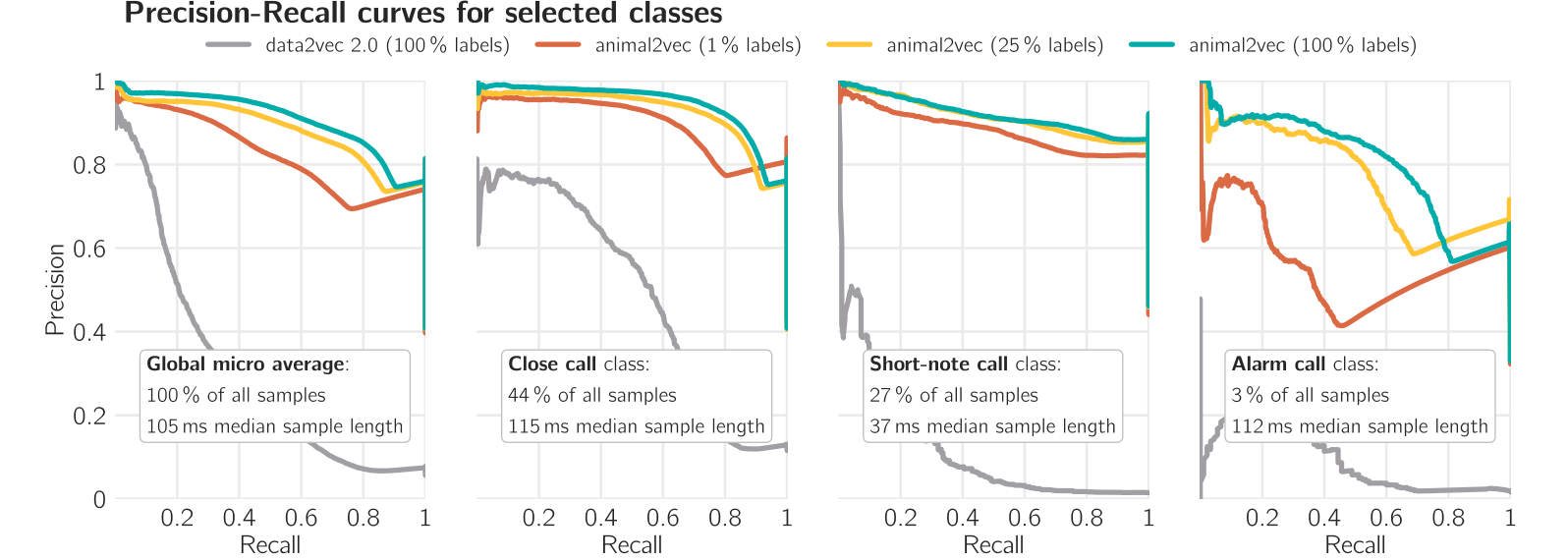
1% of fine-tuning labels
Micro-average AP: 0.83
100% of fine-tuning labels
Micro-average AP: 0.91
What stayed the same?
Pretraining used the full 1,068 h.
A strong published result is not a transfer guarantee
Evidence supplied by the paper
MeerKAT experiments and the separately pretrained birdsong transfer experiments.
Evidence your project still needs
Performance on recordings representative of your species, site, devices, and target labels.
Name one way your data differ from the data used to train the model you plan to use.
Paper, workshop package, and “modern” recipe
| Name | Meaning in these slides |
|---|---|
| animal2vec, original paper | Scientific method and reported experiments |
a2v2 Python package | The supplied native-PyTorch workshop implementation |
configs/MeerKAT/ | Animal2Vec 1.0 reproduction-oriented configurations |
configs/modern/ | A different, opt-in architecture/checkpoint family |
Put the complete inference path together
Interactive example requires JavaScript.
At which stage do we obtain embeddings? At which stage can a threshold change the result?
Long recordings are processed in bounded segments
Three audio choices to check before inference
Sample rate
Inference resamples to the checkpoint’s rate. It cannot restore frequencies lost by that conversion.
Channels
The default averages channels. A selected channel uses a zero-based index.
Model vocabulary
A checkpoint only scores the labels its output head was trained to predict.
“Good enough” depends on the research question
Missed events
Could hide rare calls, interactions, or behavioural contexts.
False positives
Could inflate call counts and create unnecessary review work.
Inspect false negatives as well as the events the model already found.
Explain the pipeline to a colleague
A new WAV file enters a fixed checkpoint.
What happens next?
Explain
Samples → local features → contextual embeddings → scores → intervals.
Distinguish
Learning weights, selecting a threshold, and interpreting a prediction.
Two minutes in pairs. Identify one remaining uncertainty.
Next: make a prediction you can inspect
After the break: prepared CoCoMo environment → CLI tour → first inference.
Threshold: the score stays, the decision changes
Interactive example requires JavaScript.
a2v2-infer MODEL.native.pt AUDIO.wav events.tsv \
  --threshold 0.50 --method avg --fusion-window-seconds 0
Raise the threshold: which weak events vanish, and which runs fragment?
Pool → threshold → join adjacent active frames
Interactive example requires JavaScript.
a2v2-infer MODEL.native.pt AUDIO.wav events.tsv \
  --threshold 0.50 --method max --fusion-window-seconds 0.10
Average can attenuate short peaks. Maximum can extend or merge nearby events. Inspect both timing and false positives.
Three linked objects: audio, events, manifest
project/
  wav/clip01.wav
  lbl/clip01.h5
  manifests/train.tsv
  manifests/valid.tsv
WAV: the recorded signal
HDF5: sample-index event intervals
TSV: files in each split
train.tsv · first line: audio root · remaining fields separated by a literal TAB
/datasets/project
wav/clip01.wav	80000
The row means 80,000 waveform samples—not 80,000 model frames. Set task.data to the manifest directory.
An event label is an interval in waveform samples
# Toy vocabulary: task.unique_labels = ["call_A", "call_B"]
# 8 kHz audio; call_A from 1.00 s up to (not including) 1.15 s
start_frame_lbl = [8000]
end_frame_lbl   = [9200]
lbl_cat         = [0]
Required arrays
Same length. Starts inclusive; ends exclusive. Label indices follow the configured vocabulary.
Do not infer “background”
A fully reviewed no-event file can have empty arrays. Missing annotations are not known negatives.
Training requires the configured audio rate. min_label_size filters HDF5 file bytes; 3032 is not a minimum number of calls.
Adapt the recipe—not the checkpoint’s geometry
| What to edit | Relevant fields | What to preserve / coordinate |
|---|---|---|
| Data and task | task.data, unique_labelsdataset.train_subset / valid_subset | Label order, complete annotations, held-out groups |
| Starting model | model.w2v_pathtask.sample_rate / conv_feature_layers | Rate and frontend must match the pretrained checkpoint |
| Compute and output | distributed_world_size, max_tokensupdate_freq, checkpoint.save_dir | Match the actual launch; use a new run directory |
| Short-run timing | max_update, freeze_finetune_updateswarmup, validation and saving intervals | A 200-update run must not inherit a 10,000-update freeze schedule |
max_tokens is a waveform-sample budget, not a file count.Department for the Ecology of Animal Societies
Communication and Collective Movement (CoCoMo) Group
A representation is not a prediction table
Embeddings
[T, D]
T time positions; D learned features.
Useful for comparison and downstream analysis.
Label scores
[T, C]
The same T positions; C trained labels.
Useful for the supervised detection task.
The coordinates are learned—not named acoustic measurements
Illustrative matrix; not a measured activation pattern.
Dimension 42 is not automatically “pitch.”
Information may be distributed across many dimensions. A coordinate can encode mixtures of signal and context.
What would you need to show before calling a feature “individual identity”?
Two different kinds of averaging
What the workshop API returns
| Attribute | Shape / type | Meaning |
|---|---|---|
result.embeddings | [T, D] | Layer-averaged frame representations |
result.probabilities | [T, C] | Independent sigmoid label scores |
result.timestamps | [T] | Frame-center times in recording seconds |
result.events | Tuple of intervals | Pooled, thresholded, fused predictions |
Arrays are returned as CPU tensors. Exact T comes from the audio geometry and endpoint trimming.
Choose the unit before you make one vector
| Unit | Question it can support | What may be lost or mixed |
|---|---|---|
| Frame | How does the sound change over time? | Many strongly correlated observations |
| Annotated or predicted event | How do individual calls compare? | Within-call temporal order after pooling |
| Fixed window | What is in a standard duration of audio? | Calls and background in the same window |
| Whole recording | How do broad soundscapes compare? | Rare brief events can be diluted |
Temporal mean pooling discards order
Interactive example requires JavaScript.
Can these two frame sequences have the same mean but different biological interpretations?
Pretrained and fine-tuned spaces answer different objectives
Pretrained representation
Learned to match teacher targets from unlabelled audio.
Fine-tuned representation
Further shaped by the chosen supervised labels.
Use the extraction path that actually exists
Supported by InferenceRunner
A native fine-tuning checkpoint with a frame head.
Returns scores, embeddings, times, and events.
A different path is required
A pure pretraining checkpoint or the checked-in modern CLS classifier.
Do not pass either to the event runner.
The archive has no dedicated embedding-export CLI. Use the Python API in the practical session.
Extract all three aligned arrays in one pass
from a2v2 import InferenceRunner
from a2v2.data import load_audio

runner = InferenceRunner("MODEL.native.pt")
waveform, sample_rate = load_audio("AUDIO.wav")
result = runner.run_tensor(waveform, sample_rate)

Z = result.embeddings.numpy()     # [T, D]
t = result.timestamps.numpy()     # [T], seconds
p = result.probabilities.numpy()  # [T, C]
Use the provided native frame checkpoint. Replace the two illustrative filenames.
An event embedding can contain surrounding context
Comparable vectors need a comparable extraction policy
| Record this | Why it matters |
|---|---|
| Checkpoint identity and hash | Different learned coordinate systems |
| Layers and temporal aggregation | Different definitions of the representation |
| Sample rate, channel, segment length | Different input and context |
| Source file and interval | Return to the actual audio |
Three ways to use the representation
Retrieve
Find examples near a known call or acoustic pattern.
Explore
Inspect structure, candidate groups, and unusual observations.
Predict
Train a separate classifier or regression model on labelled outcomes.
Retrieval and exploration can be unlabelled. A labelled downstream classifier is supervised learning.
Leave this afternoon with a traceable analysis dataset
Choose one unit and one metadata field you will inspect first.
Department for the Ecology of Animal Societies
Communication and Collective Movement (CoCoMo) Group
Every vector needs an observation record
| row_id | source_file | start_s | end_s | unit | context |
|---|---|---|---|---|---|
| event_001 | rec_017.wav | 12.30 | 12.48 | event | 10 s segment |
| event_002 | rec_017.wav | 16.10 | 16.22 | event | 10 s segment |
| event_003 | rec_104.wav | 4.80 | 5.16 | event | 10 s segment |
Illustrative schema—not actual participant recordings.
The unit determines the scientific comparison
Call-level question
One interval per call. Compare examples while tracking individual, session, and detector origin.
Soundscape question
One fixed window per observation. Keep duration and sampling policy consistent.
Which level will your result generalize to: another frame, recording, individual, or site?
Pool only the frames assigned to your interval
# Z: [T, D]; t: frame-center timestamps in recording seconds
# start_s and end_s come from a declared annotation/detection policy
inside = (t >= start_s) & (t < end_s)
if not inside.any():
    raise ValueError("No frame centers fall inside this interval")
z_event = Z[inside].mean(axis=0) # [D]Very short intervals may contain no frame center: flag them, rather than silently producing NaNs.
Your detector helps decide which observations exist
Missed calls
Will be absent from a prediction-selected repertoire.
False positives
May appear as a convincing “new cluster.”
Keep the original recording clock
Store both the source interval and the extraction segment/context policy.
Three operations often called “normalization”
| Operation | What it changes | Use it deliberately |
|---|---|---|
| Waveform normalization | The model’s audio input | Part of the extraction pipeline |
| L2-normalize each vector | Each observation’s overall vector length | Makes direction, rather than magnitude, central |
| Scale each feature column | Relative weight of different dimensions | Changes distances and fitted projections |
“Similar” depends on the distance you choose
Interactive example requires JavaScript.
For your question, could vector magnitude carry useful information—or a nuisance factor?
Join metadata by identity, not by row order
features
  row_id  → vector

metadata
  row_id  → file, interval,
            individual, site,
            device, session
Check the join.
Are IDs unique?
Did any rows disappear?
Are there unexpected duplicates?
Can three random rows be traced to audio?
Keep missing metadata explicitly missing; do not invent individuals, sites, or devices.
Save enough information to repeat the extraction
Model / processing
Checkpoint hash, package snapshot, layer policy, rate, channel, segment length, aggregation.
Observation / selection
row_id, source file, interval, annotation or detector origin, threshold/fusion settings.
analysis_bundle/
  embeddings.npy        # rows identified by rows.csv
  rows.csv              # row_id, source interval, metadata
  extraction.json       # checkpoint and processing provenance
Proposed export convention for the practical—not a built-in CLI output schema.
More rows do not automatically mean more evidence
Many frames from one call
Useful temporal detail.
Not many independent calls.
Many calls from one deployment
Useful repeated observations.
Not many independent sites.
Same coordinates; a different explanation
Interactive example requires JavaScript.
Reveal the colours by call group, site, and device. Which interpretation survives?
Freeze a comparison policy before comparing methods
A method comparison is uninterpretable when the underlying observations also change unnoticed.
Ready for nearest-neighbour search?
| Check | Required answer |
|---|---|
| What is a row? | One declared frame, event, window, or recording |
| Which space? | One checkpoint and one extraction/preprocessing policy |
| Where is the sound? | Source file + interval + stable row ID |
| What could confound similarity? | At least two biological or technical metadata fields |
Pick one query observation. Explain what would count as a useful neighbour.
Test the interpretation.
Department for the Ecology of Animal Societies
Communication and Collective Movement (CoCoMo) Group
Start with the question—not the plotting function
| Your question | First tool | Its immediate output |
|---|---|---|
| What resembles this example? | Nearest neighbours | A ranked set of observations |
| What directions contain variation? | PCA | Linear coordinates and explained variance |
| What is locally neighbouring? | UMAP | A neighbourhood-oriented layout |
| Can examples be grouped? | Clustering | Candidate assignments |
| Which examples are unusual? | Outlier scoring | A ranking for inspection |
Nearest neighbours: retrieve first, interpret second
Interactive example requires JavaScript.
In your real dataset: inspect the audio, remove self-matches, and avoid near-duplicate segments.
PCA chooses directions that retain variation
Interactive example requires JavaScript.
A PCA map is a summary, not the complete space
What to read
Which differences appear along each axis?
How much variance do these axes retain?
What not to conclude
Large variation is not automatically important biology.
Two dimensions need not preserve all useful distinctions.
UMAP begins from relationships between neighbours
Interactive example requires JavaScript.
The graph below is a schematic. No UMAP fit is computed in this slide.
A UMAP island is not a discovered call category
Useful
Explore local neighbourhoods.
Inspect examples.
Compare metadata and parameter choices.
Not established by the map
Biological category count.
Meaning of empty gaps.
Original-space density or global distance.
k-means: ask for K groups, then get K groups
Interactive example requires JavaScript.
Cluster assignments are fitted in the 12-D feature space. The PCA coordinates only display them.
Density-based grouping can leave points unassigned
Interactive example requires JavaScript.
Grey observations are marked noise. “Noise” here is an algorithmic status—not a biological annotation.
A candidate group needs an audit
| Inspect | Why |
|---|---|
| Typical examples and boundary cases | A centroid alone can hide variation |
| Individual / session / device / site | Technical or sampling factors may explain the group |
| Different parameters and resamples | A fragile partition may not support a stable interpretation |
| Independent annotated observations | Test the proposed biological interpretation |
What observation would make you reject your current interpretation of a cluster?
Outliers are candidates for inspection
Interactive example requires JavaScript.
Rare vocalization? Corrupted file? Unusual background? Annotation mistake? Listen before naming it.
Turn exploration into an annotation decision
Seek coverage
Inspect diverse and underrepresented regions.
Keep a comparison sample
Do not review only what the current model considers unusual.
One visible structure can support several stories
Interactive example requires JavaScript.
State a hypothesis with no labels. Then reveal site, device, and call group in that order.
Change a decision; check whether the finding survives
| Decision to perturb | Question to ask |
|---|---|
| Model / layer choice | Does the proposed structure depend on one representation? |
| Aggregation / normalization / metric | Does the observation definition change the conclusion? |
| Projection / clustering settings / seed | Is the visible or assigned structure stable? |
| Held-out sessions / individuals / sites | Does the interpretation survive a new context? |
Next: the mystery-dataset exercise
Before metadata reveal
Describe the structure.
Inspect examples.
Write a testable hypothesis.
After metadata reveal
Compare alternative explanations.
Revise the hypothesis.
Identify the next validation step.
Use the map to ask better questions
A neighbour is a retrieval result.
A cluster is a candidate grouping.
An outlier is a review priority.
Which analysis will you try first—and what would convince you that it is useful?